Thursday, October 28, 2021

Use Groovy to create a Jenkins Parametrized Free-Style Project

Motivation

The Jenkins Java API is a rich and endless source of useful functionality. It is also complex and unless you are a contributor that has built a Jenkins plugin, it is unlikely that you needed to deal with it directly. Nonetheless, even if you are not developing a plugin it is sometimes worth taking a look at how to use it in a simpler way. This simpler way is through Groovy the native scripting language of Jenkins. In my work with life-science Jenkins applications I work primarily with free-style parametrized jobs, and so in this post I will demonstrate how we can use selected parts of the Java API to programmatically create and parametrize a Jenkins job using just the Jenkins Groovy script console.

We can parametrize Jenkins jobs with some standard parameter types (String, Text, Boolean, File etc.) as well as with parameters that are contributed from installed plugins (for example Active Choices).

All of these parameters are defined as Jenkins extension points, and we can use the Jenkins API to discover them.
From the Jenkins API documentation we learn that 'The actual meaning and the purpose of parameters are entirely up to users, so what the concrete parameter implementation is pluggable. Write subclasses in a plugin and put Extension on the descriptor to register them.'

How to find the Jenkins available parameter types

To query for the available types we use the following Groovy code that calls the Jenkins Java API. Note that all of the example Groovy code in these examples can be executed from the Jenkins script console

ep=hudson.ExtensionList.lookup(hudson.model.ParameterDefinition.ParameterDescriptor)
ep.each{
println it.getDisplayName()
}

Executing this script produces the following results on my Jenkins instance:

We essentially lookup in the Jenkins registered extensions, those that are of a specific class. Each parameter type has a corresponding ParameterDescriptor class that describes it. We then use the getDisplayName method to get the human readable names of these parameters (otherwise we get the class name of the plugin contributing the parameter) .


A look at a parametrized job structure

The ParametersDefinitionProperty list


When we examine the configuration file (config.xml) of a parametrized job, we find that all of the job parameters are nested into a ParametersDefinitionProperty that acts as a container for all of the job parameter definitions


From the Jenkins API documentation we learn that '
ParametersDefinitionProperty Keeps a list of the parameters defined for a project.When a job is configured with ParametersDefinitionProperty, which in turns retains ParameterDefinitions, user would have to enter the values for the defined build parameters. 


Programmatic Job parametrization


It is possible to both create and parametrize a job programmatically, without ever opening the job configuration form 
 
create a new job, lets call it 'MyTest01'
myJenkins=jenkins.model.Jenkins.instance
myJenkins.createProject(FreeStyleProject,'MyTest01')
job1=myJenkins.getJob("MyTest01")
Add a ParametersDefinitionProperty to the job
job1.addProperty(new hudson.model.ParametersDefinitionProperty())
Now the job is parametrized!
println 'IsParametized:'+job1.isParameterized()
Result
IsParametized:true

Now we have a parametrized job, but have not defined any parameters yet. 

For simplicity, in this example we have used the null parameter constructor for ParametersDefinitionProperty. However, the constructor allows passing a list of parameter definitions, so if we add a list of ParameterDefinitions we can add the required project parameters!


Programmatic creation and parametrization of a free-style job

A complete example


We will now present a complete step-by-step example where we not only create a parametrized job but also add a couple of parameters. 

To make this example even more interesting, one of the parameters will be an Active Choices parameter, and in the process we'll show how you can add the required Groovy script for the Active Choice parameter configuration.

The following code is a complete example of creating and parametrizing a free-style job programmatically. 


Tasks

  1. Create a new Jenkins job
  2. Construct 2 parameters
    1. A simple String parameter
    2. An Active Choice parameter (with a secure groovy Script)
  3. Construct a ParametersDefinitionProperty with a list of 2 parameters
  4. Add the ParametersDefinitionProperty to the project
  5. Print some diagnostics
The task list labels also match the labels identifying the code fragments in the table below to make it clear what the code fragments do. 

a
jenkins=jenkins.model.Jenkins.instance
jenkins.createProject(FreeStyleProject,'MyTest01')
job1=jenkins.model.Jenkins.instance.getJob("MyTest01")

b.i
pdef1=new StringParameterDefinition('Myname', 'IoannisIsdefaultValue', 'MyNameDescription')
b.ii
sgs=new org.jenkinsci.plugins.scriptsecurity.sandbox.groovy.SecureGroovyScript("""return['A','B','C']""", false, null)
acScript=new org.biouno.unochoice.model.GroovyScript(sgs,null)
pdef2=new org.biouno.unochoice.ChoiceParameter ('AC_01TEST', 'ACDdescription','boo123', acScript, 'PARAMETER_TYPE_SINGLE_SELECT', true,2)

c,d
job1.addProperty(new hudson.model.ParametersDefinitionProperty([pdef1,pdef2]))
e
println 'IsParametized:'+job1.isParameterized()
println job1.properties
job1.properties.each{
  println it.value.class
  println 'Descriptor:'+it.value.getDescriptor()
  if( it.value.class==hudson.model.ParametersDefinitionProperty){
    println 'Job Parameters'
    println it.value.getParameterDefinitionNames()
    it.value.getParameterDefinitionNames().each{pd->
      println it.value.getParameterDefinition(pd).dump()
    }
  }
}
Result
IsParametized:true
[com.sonyericsson.hudson.plugins.metadata.model.MetadataJobProperty$MetaDataJobPropertyDescriptor@5ba29d96:com.sonyericsson.hudson.plugins.metadata.model.MetadataJobProperty@23d5994d, com.sonyericsson.rebuild.RebuildSettings$DescriptorImpl@52e43430:com.sonyericsson.rebuild.RebuildSettings@56c0e80c, hudson.model.ParametersDefinitionProperty$DescriptorImpl@1b2facb8:hudson.model.ParametersDefinitionProperty@6054a6c5]
class com.sonyericsson.hudson.plugins.metadata.model.MetadataJobProperty
Descriptor:com.sonyericsson.hudson.plugins.metadata.model.MetadataJobProperty$MetaDataJobPropertyDescriptor@5ba29d96
class com.sonyericsson.rebuild.RebuildSettings
Descriptor:com.sonyericsson.rebuild.RebuildSettings$DescriptorImpl@52e43430
class hudson.model.ParametersDefinitionProperty
Descriptor:hudson.model.ParametersDefinitionProperty$DescriptorImpl@1b2facb8
Job Parameters
[Myname, AC_01TEST]
<hudson.model.StringParameterDefinition@125d74 defaultValue=IoannisIsdefaultValue trim=false name=Myname description=MyNameDescription>
<org.biouno.unochoice.ChoiceParameter@35c83a1d choiceType=PARAMETER_TYPE_SINGLE_SELECT filterable=true filterLength=2 visibleItemCount=1 script=GroovyScript [script=return['A','B','C'], fallbackScript=] projectName=null randomName=boo123 name=AC_01TEST description=ACDdescription>

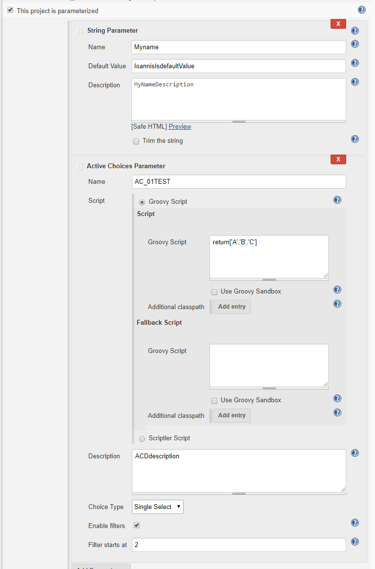
Examine the configuration of the newly created project


We will finally review our programmatic creation with the aid of a standard job configuration page. Find the job and click the configure action on the left panel.


Note that the 'Build with Parameters' Form UI is not updated until the project definition is saved to disk. 

Once we 'Apply' or 'Save' the job configuration we can then review the build form UI with the programmatically created parameters.

Summary

We can use Groovy scripts to interact with the Jenkins Java API in many different ways. This is a simple example, but clearly demonstrates the popular concept of  'configuration-as-code' and also helped me to understand some of the Jenkins Java API used with parametrized jobs.

Free-style parametrized jobs are key components to life-science Jenkins applications, and using the Jenkins API allows us to reuse subsets of the job parameters in an ad-hoc way to build reusable interactive components (more details here: imoutsatsos/JENKINS-JOB_PARAM_ASSEMBLER: Utility job for replicating parameters across freestyle jobs (github.com)).


Friday, February 8, 2019

The 'snake pit' of Anaconda and R-reticulate

Background

The R-Studio team is making an important contribution with the 'reticulate' package for reusing Python modules in R. The reticulate package makes it possible to embed a Python session within an R process, allowing you to import Python modules and call their functions directly from R. If you are an R developer that uses Python for some of your work or a member of data science team that uses both languages, reticulate can dramatically streamline your workflow.[1]

Into the 'snake pit'

The last few days I have been trying to do some data analysis using the 'umap' dimensionality reduction and visualization algorithm [3]. My preferred data analysis environment is R as it is easy to integrate R-scripts into our data management and analytics workflow using Jenkins-LSCI.[4]

It all started innocently enough, as I decided to use the flipDimensionReduction package[2] (from Displayr), a package that I had used previously to create t-SNE visualizations of multi-dimensional data. The Display r dimension reduction function also supports using the UMAP algorithm as an alternative to t-SNE

However, the use of the UMAP option requires the external python module 'umap-learn'. And this is where my adventure begun..

A quick test (code shown below) from within R-Studio on my desktop (a Win-10 laptop, R v3.5.2, Anaconda distribution of Python 3.6) worked flawlessly and I was very encouraged!

 library(flipDimensionReduction)  
 library(reticulate)
 ## Read in data set file and apply dimension reduction algorithm 
 redData<- read.csv('http://localhost:8080/job/UTIL_CSVDATA_QUERY/39/artifact/customQuery_1548177063100.csv')   
tSNE_p30<-flipDimensionReduction::DimensionReductionScatterplot("t-SNE", redData, data.groups = redData$LABEL, perplexity = 30, seed = 3456)  
 ##To use the UMAP algorithm simply replace 't-SNE' with 'UMAP'  
 umap_p30<-flipDimensionReduction::DimensionReductionScatterplot("UMAP", redData, data.groups = redData$LABEL, perplexity = 30, seed = 3456)  

Goal: Run flipDimensionReduction with UMAP from an R-Script

Now, let's describe the environment that I would really like to run this
  1. Windows 2008 server
  2. R v 3.5.2
  3. Anaconda distribution of Python 2.7.15
  4. The R-script has to run from the command line and not from within R-Studio

[Failed] Update Anaconda Distribution from Python 2.7 to Python 3.x

Given that the Anaconda Navigator and Python installations on the Windows server were both older versions, I decided to update them using the recommended conda command [5,6]

conda install anaconda


However, this did not work as expected (I was expecting an update to the latest version of Python). It seems that all I got was an updated version of the Anaconda Python 2.7.15 distribution

[Success] Creating a 'conda' Python 3.7 environment'

I then decided to create a new conda environment, 'py37' with the latest version of Python 3.7. This was done from the user interface of the Anaconda Navigator and completed successfully.

[Failed] Anaconda Navigator: Add the 'conda-forge' channel

This is the repository (channel) that hosts the 'umap-learn' module. I proceeded to add it from the user interface of the Anaconda Navigator. Then we need to click 'Update Index...' This operation hung the Anaconda Navigator ...forever! Now, every time Anaconda starts, it hangs while displaying 'Adding featured channels...' I have to kill the python process to exit!

Apparently this is a known (and as of now, 2/7/2019, unresolved) issue

[Success] Command line installation of  'umap-learn' 

Thankfully, the Anaconda 'py37' environment console is still functional and so I continued the installation from the command line

conda install -c conda-forge umap-learn
conda list

The 'list' command displays all the 'py37' installed modules, and it displays the 'umap-learn' package as correctly installed.

Is it time to rejoice that we've made it out of the 'snake pit' of module updates and installation? The joy is being able to use the UMAP algorithm from R. Let's give it a try.

[Failed]: Attempt 1: Using 'umap-learn' from R

Now that the 'umap' package was installed it was time to try it from R.

Given that I had two environments for python  (the 'base' python 2.7.15 without the 'umap-learn' package, and the 'py37' with the 'umap-learn' module) I followed the instructions for configuring the python 'py37' environment for use by R[7].

The instructions suggest that 'reticulate' 'can bind to any of these Python versions' by one of several ways.

I decided to use the use_python("PATH_TO_PYTHON") 'reticulate' function.

> library(reticulate)
> use_python("D:/DEVTOOLS/Anaconda2/envs/py37")

> py_config()
python:         D:\DEVTOOLS\ANACON~1\python.exe
libpython:      D:/DEVTOOLS/ANACON~1/python27.dll
pythonhome:     D:\DEVTOOLS\ANACON~1
version:        2.7.15 |Anaconda, Inc.| (default, Dec 10 2018, 21:57:18) [MSC v.1500 64 bit (AMD64)]
Architecture:   64bit
numpy:          D:\DEVTOOLS\ANACON~1\lib\site-packages\numpy
numpy_version:  1.15.4

python versions found: 
 D:/DEVTOOLS/Anaconda2/envs/py37/python.exe
 D:\DEVTOOLS\ANACON~1\python.exe
 D:\DEVTOOLS\Anaconda2\python.exe
 D:\DEVTOOLS\Anaconda2\envs\py37\python.exe
> 

But wait, py_config reports Python version is 2.7.15, not what I expected. What's happening here?

It seems that despite the use_python() directive, 'reticulate' still binds the older version of python (which I don't want since it does not include the 'umap-learn' module)

After none of the suggested 'reticulate' functions that dynamically define a Python environment to use worked, I decided to specify the Python location from a system environment variable.

[Failed] Attempt 2: Using 'umap-learn' from R

Add a new Windows system environment variable:
RETICULATE_PYTHON="D:\DEVTOOLS\Anaconda2\envs\py37\python.exe"

Start a new session of R. Apparently a session can only import a single Python environment and it can not be reset. So always test by starting a new R console session.
> library(reticulate)
> py_discover_config()
python:         D:\DEVTOOLS\Anaconda2\envs\py37\python.exe
libpython:      D:/DEVTOOLS/Anaconda2/envs/py37/python37.dll
pythonhome:     D:\DEVTOOLS\ANACON~1\envs\py37
version:        3.7.1 (default, Dec 10 2018, 22:54:23) [MSC v.1915 64 bit (AMD64)]
Architecture:   64bit
numpy:           [NOT FOUND]

NOTE: Python version was forced by RETICULATE_PYTHON
> import("umap-learn")
Error in py_module_import(module, convert = convert) : 
  ModuleNotFoundError: No module named 'umap-learn'
> 

So, now I forced 'reticulate' to use the version of Python I wanted, but it still can't find the module!

[Success]What is your real name 'umap-learn'?

More investigation revealed that the 'umap-learn' module although appears in the 'conda list' with the name 'umap-learn' it is really named 'umap' (in the envs\py37\Lib\site-packages folder) so the import fails!

Let's retry importing with the 'umap' name.

> import("umap")
Module(umap)

[Failed] Attempt 3: Using 'umap-learn' from R (NumPy version?)

So at this point I'm finally able to import the desired module. Let's try to use it.

> redData=read.csv('http://localhost:8080/job/UTIL_CSVDATA_QUERY/39/artifact/customQuery_1548177063100.csv')
> library(flipDimensionReduction)
> tSNE_p30=flipDimensionReduction::DimensionReductionScatterplot("t-SNE", redData, data.groups = redData$LABEL, perplexity = 30, seed = 3456)
> umap_p30=flipDimensionReduction::DimensionReductionScatterplot("UMAP", redData, data.groups = redData$LABEL, perplexity = 30, seed = 3456)
Error in py_call_impl(callable, dots$args, dots$keywords) : 
  Evaluation error: Required version of NumPy not available: installation of Numpy >= 1.6 not found.

As of this writing NumPy is at version 1.15.4 and I have the most recent version. What is this?
Well, after some more investigation and assistance from StackOverflow this is another unresolved issue with 'reticulate' [8]

The suggestion was to downgrade the version of 'numPy' but this did not work for me. What worked was the suggestion from gitHub: https://github.com/rstudio/reticulate/issues/367

The suggested solution is to add the Anaconda `libraries\bin` directory to the path prior to initializing Python.

[Success] Attempt 4: Initializing Python with path to libraries


#now some environment hacks to get around known issues with 'reticulate'
# see https://github.com/rstudio/reticulate/issues/367
> Sys.setenv(PATH= paste("D:/DEVTOOLS/Anaconda2/envs/py37/Library/bin",Sys.getenv()["PATH"],sep=";"))
> library(reticulate)
> import("umap")
Module(umap)
> py_config()
python:         D:\DEVTOOLS\Anaconda2\envs\py37\python.exe
libpython:      D:/DEVTOOLS/Anaconda2/envs/py37/python37.dll
pythonhome:     D:\DEVTOOLS\ANACON~1\envs\py37
version:        3.7.1 (default, Dec 10 2018, 22:54:23) [MSC v.1915 64 bit (AMD64)]
Architecture:   64bit
numpy:          D:\DEVTOOLS\ANACON~1\envs\py37\lib\site-packages\numpy
numpy_version:  1.15.1
umap:           D:\DEVTOOLS\ANACON~1\envs\py37\lib\site-packages\umap\__init__.p

NOTE: Python version was forced by RETICULATE_PYTHON

> library(flipDimensionReduction)

> redData= read.csv('http://localhost:8080/job/UTIL_CSVDATA_QUERY/39/artifact/customQuery_1548177063100.csv')   
> tSNE_p30=flipDimensionReduction::DimensionReductionScatterplot("t-SNE", redData, data.groups = redData$LABEL, perplexity = 30, seed = 3456)  

> ##To use the UMAP algorithm simply replace 't-SNE' with 'UMAP'  
> umap_p30=flipDimensionReduction::DimensionReductionScatterplot("UMAP", redData, data.groups = redData$LABEL, perplexity = 30, seed = 3456)  
> umap_p30
This last command uses the print function of the umap_p30 object to create an interactive UMAP web-page.

UMAP Interactive

'Out of the snake pit' What have I learned?

So, finally I have the reduction algorithm running in R with the UMAP option. And yes, it uses the 'reticulate' package to import the latest version of Python and its installed modules.

But the experience of getting this to work was anything but smooth!
  • The 'reticulate' R package issues seemed to have been known for several months, but still remain unresolved. 
  • The 'reticulate' functions for binding to specific Python versions and environments, and for reolving library class paths, did not work as expected. These seem fundamental to the usage of the package. If they did work, the process would have been a lot smoother.
  • Some of the issues seemed total 'red-herrings' and the error messages not helpful (see issue of NumPy version). 
  • The issue of the actual 'umap' module name vs. the name used to install it is still unclear to me, but perhaps someone with more experience in Python can explain why.
  • Finally, the Anaconda Navigator exhibited a crash behavior from which it never recovered. I think I will stick with the Anaconda command prompt.
In the end, I've put these notes together in the hope that they'll help someone else to setup and troubleshoot this important functionality of 'reticulate' in less time than it took me.

References

  1. RStudio 1.2 Preview: Reticulated Python https://blog.rstudio.com/2018/10/09/rstudio-1-2-preview-reticulated-python/
  2. flipDimensionReduction by Displayr:https://rdrr.io/github/Displayr/flipDimensionReduction/
  3. UMAP: Uniform Manifold Approximation and Projection for Dimension Reduction https://arxiv.org/abs/1802.03426
  4. Continuous Integration of life-science data workflows with Jenkins https://github.com/Novartis/Jenkins-LSCI
  5. Updating Anaconda to Python 3.6 https://support.anaconda.com/customer/en/portal/articles/2797011-updating-anaconda-to-python-3-6
  6. Updating Anaconda: https://stackoverflow.com/questions/45197777/how-do-i-update-anaconda
  7. Python Version Configuration: https://rstudio.github.io/reticulate/articles/versions.html
  8. Using Python in R with reticulate package - Numpy not found
  9. https://stackoverflow.com/questions/54069769/using-python-in-r-with-reticulate-package-numpy-not-found

Wednesday, January 2, 2019

External Libraries for Active Choices

Motivation

The question 'How can I use jar-X or library-X in my Active Choice Groovy script ' is frequently asked. Using external java libraries in Groovy is one of the most useful features of the language, and so we need to explore how to easily make external libraries accessible to the Groovy scripts used to generate Active Choice parameters.

A Note on Jenkins Security

Groovy script execution in Jenkins is increasingly coming under scrutiny by the Jenkins security team. Several things that were easy to do with Groovy in Jenkins are now restricted, or next to impossible, due to security restrictions. As a result, some of the recommendations below may or may not work in future Jenkins versions and with future upgrades to the various plugins.

In later versions of Jenkins (v2.361.x and perhaps others) the approaches described below for v222.x have been blocked by security and JDK11 requirements. I will post any new information I find out, but for the time being, consider this limitation if you are trying to use external libraries with Active Choices in more recent versions of Jenkins.

External Libraries for Active Choices (Jenkins v2.222.x)


Options for Jenkins v2.222.x and earlier
There are at least three different ways we can employ to include external Java/Groovy libraries in the classpath of the Active Choices script.

  1. Configure an 'Additional Classpath' in the Active Choices Parameter Groovy script. 
    • Place the required library on the classpath folder on the Jenkins server. You can configure the additional classpath using tokenized variables accessible to the Active Choices script
    • I frequently place external libraries in a dedicated folder under the JENKINS_HOME/userContent folder. For example, a classpath to the H2 java database jar can be configured as $JENKINS_HOME/userContent/lib/h2-1.3.176.jar
    • Note that additional Classpaths seem to be discouraged in the latest Groovy Plugin. See https://issues.jenkins-ci.org/browse/JENKINS-43844
  2. Use Grape, the JAR dependency manager embedded into Groovy. The @Grab Groovy annotation dynamically fetches the required java library
  3. Place the required library in an external java libraries folder. Java (and Groovy) use these classpaths by default
    • In the Jenkins Groovy Console execute: println System.getProperty("java.ext.dirs")  to review what folders are used for external libraries
    • The path to all external java folders can be discovered by examining the 'java.library.path' property in the System Information link on the 'Manage Jenkins' page
    • Placing the required jar in one of the available java.library.path folders should work well for most cases and should be considered secure since you'll need admin access to have the ability to copy the jars to the appropriate location and restart the Jenkins server for these changes to take effect.

In Conclusion

As always, there are multiple ways to achieve  this programming requirement. Hopefully, one of these works for you! I will be happy to hear of other alternatives that you may discover or have used. Please, leave them in your comments and I can incorporate them in the blog entry.

References


  1. Jenkins Active Choices Plugin
  2. Grape dependency manager in Groovy
  3. BioUno: Jenkins and DevOps Tools for Life Sciences


Wednesday, October 10, 2018

Jenkins Active Choices & Dynamic JavaScript Generation

Motivation

Many Jenkins job build forms using Active Choices parameters also include dynamically generated JavaScript. JavaScript is included into the build form in either of two ways:

  1. Directly from an Active Choice Reactive Reference parameter, returning an HTML <script> element or
  2. From an Active Choice Reactive Reference parameter reading a JavaScript file from the Jenkins server (either in JENKIND_HOME/userContent or JOB_NAME/BuildScipts folder of the job) and returning HTML with the file contents in the <script> element.

In addition, many job builds publish an interactive HTML build report that imports and uses JavaScipt libraries and scripts. To preserve the long term functionality for these reports (even as the custom JavaScript code may evolve) I also archive the custom JavaScript used in these forms, so each report uses a version of the script with  which it was intended to work with

As an example, I use the Openseadragon.js library (for web-viewing high resolution zoomable images) in a number of build forms. A Jenkins Active Choices Reactive Reference parameter rendered as an HTML <script> element that uses the OpenSeadragon.js library to render biological images on a Jenkins Build Form is shown below:

Initially, specific versions of this library were hard-coded into the Active Choice parameter groovy scripts and the text templates.

I revised the design strategy so that we can have a single, dynamic reference to the latest OpenSeadragon library that can then be referenced and used by Active Choice parameters, scripts and HTML templates

Overall Strategy


Implementation requirements

Global Jenkins Property

The library version is maintained as a global Jenkins parameter. We will use this as the single reference that can update all other occurrences of the library. So in the Jenkins Configuration we setup a Global Variable like:
OPENSEADRAGON_JS=openseadragon-bin-2.4.0

Active Choices Reference Parameter (on build form)

This dynamic parameter (code gist here) performs the following functions:
  • Parametrizes the JavaScript template to create the code used in the build form
  • Loads the JavaScript into the build form
  • Writes this dynamic JavaScript to a custom session specific WORKSPACE as the Report JavaScript  (if it will be included in the build generated HTML report)

Scriptlet Build Step: Generates HTML from Template

  • Parametrizes the HTML  Report template
  • Writes the generated dynamic HTML to an HTML Report File. (Note that in some cases the HTML Report loads and uses the JavaScript file generated by the Active Choices parameter above)
  • Code gist here

Scriptlet Build Step: Copy Session JavaScipt to Job Workspace 

  • Copies the session specific JavaScript file to the job workspace so that it can be archived and used in the build HTML report
  • Code gist here


Monday, September 17, 2018

RStudio Data Structure Helpers

Frequently an R function outputs a data object that has internal structure and perhaps other nested objects.The internal structure of an R object can be reviewed in more detail with the structure command

str(object)

Furthermore, RStudio provides multiple helpers for accessing nested structures in the generated objects. Let's quickly review what can be done.

Start with the Global Environment viewer

The right pane of an RStudio R session displays the session Global Environment.


The icons on the right of the list of session objects (indicated in the screeenshot by blue and yellow arows) allow you to easily review and drill down to the structure of these objects.

For example, clicking on the table-like icon opens a tab in RStudio with a tabular display of the object (usually a data frame)

Complex (non-Tabular) objects


Complex objects are identified by their type.

For example, the tsneT1 object is of type '2Dreduction', and we can reveal its complex structure by clicking on the magnifying glass icon to the right of the list. This opens a new RStudio editor tab and displays the following:

Reviewing elements of complex objects 

We can still further review the elements of the tsne complex object.
Hovering over the elements of the complex tsneT1, object reveals a 'console code' symbol to the right.
Clicking on the 'embedding' list element enters in the console the R command for exploring this element's structure.

Exporting elements of complex objects


Finally, we may need to export one of the elements of the complex object for further analysis. In my case, I was interested in exporting the t-SNE embeddings (dimenstions) so I used the following command

## Export TSNE and labels
write.csv(tsneT1[["embedding"]], file.choose(), row.names=LabelsT1)

This exported the tsneT1 embeddings to a file on the file  system

In Summary

These are some quick tips on how to use the RStudio structure viewing tools for exploring R object data structures for debugging and analysis purposes. I hope you find them useful

Wednesday, June 7, 2017

Librarians and Triple-Eye-Eff to the rescue of scientific imaging

Somewhat unrecognized by us life-scientists, when it comes to delivering impressive images and associated annotations in an interoperable manner, across diverse media types and document repositories, librarians and cultural collection curators are running circles around us!

Welcome to the International Image Interoperability Framework or IIIF (Triple-Eye-Eff) for short. When I started exploring image servers for biological imaging (specifically around high content screening applications) it was not long before I started coming across references to IIIF and its associated technologies of image servers, viewers, annotation servers and compatible APIs. The technologies are open source, well-accepted, firmly established, and supported by a talented group of technical experts that call museums and libraries home to their daily work. Importantly, IIIF practitioners meet at some great places. The 2017 IIF Conference is taking place at the Vatican this week (June 5-9, 2017).

After reviewing some of the IIIF community goals, I see that the they align almost perfectly with those of biologists and life scientists working with scientific image collections.
  • A scientific study creates a collection of high resolution images similarly to a collection of images created by scanning the pages of a manuscript in a library collection.
  • Scientist require delivery of images at various resolutions (thumbnails for quick inspection and high resolution for detailed inspection), for dynamic viewing similarly to how a curator would examine the scanned pages of an ancient manuscript. The IIIF-Image API specifies the web service endpoints that return an image in response to a standard HTTP or HTTPS request.
  • The sequence and order of the images is important. A book is an ordered collection of pages, starting with a cover page and followed by an ordered  sequence of pages. Similarly, images from a HCS assay are organized as "plate collections" each with a specified order of columns and rows. The IIF Presentation API defines the structure and layout of a complex image-based object using JSON-LD (linked data) notation.
  • Scientific images are best understood in context. The ability to add annotation and metadata to any collection or individual image is critical. IIIF accomplishes this through the IIIF Annotation API which is an extension of the Open Annotation (now Web Annotation) data model. I IIF web viewer/client tools (like the Mirador viewer, developed by Stanford University) support direct user highlighting and annotation of an image area of interest. 
  • Scientist need to accurately communicate experimental results. The ability to draw attention to specific features in the image by adding graphical annotations is a necessity. Many IIIF based tools support this functionality, and allow users to add labels and markings (geometric shapes, arrows, hand drawn markings etc) as overlays to the images.
  • Scientific images collected in different repositories and by different technologies frequently need to be shared and integrated with other types of information. A central role of IIIF technologies is to provide the APIs and framework to share these image collections across multiple sites.

I should mention that IIIF has not gone completely unnoticed outside the realm of cultural collection curators. There are already a number of life-science and earth-science projects and research applications that use at least part of the IIIF technologies.

Here are a few examples:

From Biology (Histology Examples)
Annotation
From Other Sciences

Despite this almost perfect alignment of goals between IIIF and scientific imaging, there are still some important functional gaps. In my preliminary evaluation, I've noticed that although there have been a few discussions on this topic, multi-spectral images are not a focus of the current IIIF specification,  Multi-spectral imaging is a core principle in biological imaging and the need to combine multiple channel images into a composite image is ubiquitous.

There are also some areas where due to my limited experience with the IIIF presentation API I have unanswered questions. For example, how does IIIF handle Z-stacks comprising a 3D image, or video frames comprising time series (time lapse imaging)? Would the framework be able to  present these time or space-related images appropriately?

My excitement for combining IIIF with my work on HCS imaging is such that I'm attending the 2017 Vatican meeting!! More notes after the meeting will come. 

Thursday, March 9, 2017

A tinyurl helps you to easily post Google Photos elsewhere

Google Photos can be a blessing and a curse. While providing some great functionality to backup, sync and organize your photos from multiple devices, Google Photos can be painful when you need to reuse your photos on some of your other favorite sites such as Pinterest, Houzz, blogging and social media sites.

Recently I was trying to put some of my Google Photos on Houzz, a site for sharing home improvement design ideas and projects. I figured I would just right click, copy the image link from Google Photos and use it in the upload widget for Houzz. This didn't work! After a few attempts I've realized that the link URL is too long to be pasted into the the file chooser text box of Explorer.

I then figured I would use the photo 'Share Link' used for sharing the image with others. I had high hopes that this link could be used to upload the image to Houzz. No, that didn't work either!

As a last ditch effort, I've tried to shorten the very long image link URL (over 600 characters!) using the tinyurl website.


The shortened URL worked like a charm!
Using the tinyurl I was able to upload the picture with the Houzz upload widget.

This could be a relatively easy workaround to the vexing problem of easily posting your Google photos to other sites. Let me know if this works for you!